International EM induction workshop 2014

International EM induction workshops

Germany 24 – 30 August 2014

IAGA (International Association of Geomagnetism and Aeronomy) is one of eight associations within IUGG (International Union of Geodesy and Geophysics) and IUGG is one of thirty unions within ICSU (International Council for Science).

The main activity of working group I.2 of IAGA is the biennial Electromagnetic Induction in the Earth Workshops, initiated in 1972. The EM induction workshops are the most important events for researchers around the world in the field of electromagnetism in geophysics.

The 22nd EM Induction Workshop in 2014 is organized by the German EM community.

Scientific Program

Please check back in early 2014 for more information on submitting abstracts and the scientific program.

Workshop Invited Reviewers

We are pleased to announce invited reviews from a range of acclaimed international scientists who are experts in their fields. These invited reviews provide a unique opportunity to hear the state-of-the-art in electromagnetic methods and applications. As in previous Workshops, these reviews will later be published.

Joint inversion of refraction and reflection seismics traveltimes data

Joint inversion of refraction and reflection seismics traveltimes data

Kaminsky Alex, Zond software

Introduction

The joint inversion method for  arrival times  of refracted and reflected waves is discussed in this paper. Nowadays this approach is  popular and widely used for solving task of deep seismic exploration. Here we consider an algorithm of forward and inverse problems  specialized for near surface  seismics.

In engineering seismics there was many attempt separation of the reflected waves for extra information. It well known that using of refracted waves only, gives too rough  velocity profile.

Unfortunately, in most cases of engineering studies, there is difficult to identify the reflected waves, because it is "noised" by other types of waves. Since the problem of identification of the reflected waves is an independent, complex direction -  and will not be considered here. Let us assume that for our task, the first breaks and the time of arrival of the reflected waves for the n-th number of boundaries are known.

Forward problem

Forward problem - calculation the first arrival times and the arrival of the reflected waves for a model with an arbitrary velocity distribution and geometry of the reflector based on the Shortest path method (Moser, 1991). This method allows us to calculate the shortest ray path for refracted waves.

The combination of minimum paths  from the source and the receiver to the reflector point allows the build path of the reflected wave for each boundary. Minimal total travel time from the source and the receiver is selected as a reflection point of the border. Using of this method removes the restriction on the complexity geometry  of topography and the  reflecting boundary and  can be used for the interpretation of engineering seismics .

Forward problem has been developed for the two types of models. In the first case velocity section defined as a set of layers with arbitrary geometry boundaries and arbitrary distribution of the velocity inside each layer. The complexity of the boundaries is controlled by nodes number. Any boundary can be reflected and refracted, or only refracted. The advantages of this model type is the possibility of joint interpretation of P and S waves in a common geometry boundaries. Also, it is convenient to use for  sparse observation systems.

In the second case, the model is divided regular mesh of cells with arbitrary velocity. Reflected boundaries are set arbitrarily and are not joined with the geometry of the cells. This type of model is useful for dense observation networks, such as seismic tomography.

Additional extra features of the algorithm includes the possibility of taking account of surface  topography,  anisotropy and the attenuation parameter.

Testing algorithm of forward problem was carried out for a number of analytical solutions and using other well known algorithms (Fig. 1). Shortest path method is based on graph theory, and has controlled accuracy, so when a sufficiently dense subdividing of boundaries could get accuracy less than 0.01 percent.

Figure 1 Calculated reflected (A) and refracted (B) travel times curves and ray paths for complex velocity model.

Inverse problem

For the inverse problem Occam inversion (Constable et all, 1987) procedure was used. The main problem with the joint inversion of velocities and geometry of boundaries is the difference of dimensions for this parameters. This negatively affects the properties of the matrix system. To reduce the dynamic range of the matrix - logarithmic norms of parameters (velocities and  local thicknesses of layers and  apparent velocities) were used.

        Using of thicknesses instead  the depths is allow to avoid the problem of boundaries intersection in the resulting model.  Also, in order to suppress  strong oscillations of geometry,   an additional parameter controls the relative speed of change for velocity and thicknesses was used. Smoothing filter is constructed differently for the two types of models. In the first case, the operator is designed separately for each layer and works in the horizontal direction.  In the second case the common filter is used for smoothing all cell's velocities and additional  - for smoothing  layer's boundary.

Algorithm testing

Inversion algorithm was tested on synthetic data (Fig.2) calculated for several types of velocity models. As a tested model - four-layer cross-section  with arbitrary boundaries and the high-velocity object inside second layer was used.

Node sampling interval for boundary correspond to twice distance between the geophones. Observing system correspond to seismic tomography with shot point at each geophone. Directly before each inversion of synthetic travel times noise component was added.

Testing was performed as follows:

·         In the first stage only first arrival times for the first and second types of models  were inverted. The horizontally layered  model with a constant velocity gradient  was used as start.

·         At  the second stage only reflected times for the first and second types of models  were inverted. The horizontally layered  model with a constant velocity  was used as start.

·         In the third stage, the joint  inversion for refracted and reflected waves data was carried out. In our experience, when working with synthetic data, to achieve acceptable data fitting, there is only  three or four iterations enough.

·         Finally, the inverted models were compared to the original.

Figure 2 Example of refracted and reflected synthetic travel times inversion. A – calculated reflection travel times data for original model C; B – calculated refraction travel times data for original model C; C – four-layers arbitrary velocity model with one reflections boundary(3); D – result of joint   reflected and refracted data inversion; E - result of refracted data inversion; F - result of reflected data inversion. Before every inversion pass, noise was added to the synthetic data.

Figure 2 shows the results of testing the algorithm for arbitrary layered model. This is a typical velocity section at engineering geophysical surveys. The upper part of the model consists of a low-velocity sedimentary rocks. The basis of the section is high-velocity rock formations.

Synthetic seismic survey consisted of 24 geophones spaced at 5 meters and  shots in each geophones point.

The inversion was carried out until the RMS did not reach a specified level of noise. For this example, only 4-5 iterations was enough. The average computation time for each inversion was  about  two minutes.

As seen from the figure 2, the best results were obtained from the joint inversion of reflected and refracted data 2D.  It is practically corresponds to the original model.  With the one hand, using of reflection data allow to get the best rays coverage (for a more reliable determination of the velocity), on the other - it is better to recover  the reflecting boundary geometry.

When the inversion carried out for reflected or refracted data separately, the model recovered considerably rougher. This is especially well seen for inversion of refracted data 2E. The lower boundary  (reflected) shifted by almost 10 meters.

Test results for a number of models have shown significant improvement in the accuracy of recovering parameters in the joint inversion. Algorithm for joint interpretation of refracted and reflected travel times data was  realized in the ZondST2D and is currently  testing with field's data.

Conclusions

Proposed algorithm can be used for processing of shallow seismic data. The joint inversion of reflected and refracted travel times data significantly improves the quality of the resulted velocity sections. Using of refracted and reflected travel times data together  allow to achieve greater depth of investigation.

Reference

1. Moser T.J., Shortest path calculation of seismic rays, Geophysics, vol. 56, no. 1, 1991.

     2. Constable S.,Parker R., Constable C. Occam's inversion: A practical algorithm for generating smooth models from electromagnetic sounding data. 1987. Geophysics 52, 289.

Software for 2d gravity and magnetic

Разработка алгоритма совместной инверсии времен прихода преломленных и отраженных волн

Каминский А.Е.

http://zond-geo.com

Введение

В работе рассматривается методика совместной инверсии времен прихода преломленных и отраженных волн.  Данное направление сейчас популярно и широко используется  за рубежом для решения задач глубинной сейсморазведки.

Основными  подходами к совместной интерпретации данных преломленных и отраженных волн являются:

• Полноволновая инверсия во временной или частотной области (Zhou et all, 2003)
• Совместная инверсия времен прихода отраженных волн и первых вступлений (Hobro et all., 2003)

Первое направление имеет ряд существенных ограничений при использовании в инженерной сейсморазведке. Второе направление, применительно к малоглубинным изысканиям, рассматривается в рамках данной работы.

В инженерной сейсморазведке уже достаточно давно совершаются попытки выделения отраженных волн для получения дополнительной информации.  Ведь как известно, использование только рефрагированных волн при интерпретации дает слишком грубое представление о скоростном разрезе (рис.1).  

К сожалению, в большинстве случаев, для данных полученных при инженерных изысканиях, выделить отраженные волны затруднительно, так как они сильно “зашумлены” другими типами волн.  Так как задача выделения отраженных волн является самостоятельным,  чрезвычайно сложным направлением -  здесь она рассматриваться не будет.  Примем, что для определенного профиля выделены первые вступления и времена прихода отраженных волн для n-го количества границ.

Рисунок 1 Результаты двумерной инверсии полевых данных сейсмотомографии на рефрагированных волнах.

Предпосылки к совместной интерпретации преломленных и отраженных волн

Основные минусы сейсморазведки на рефрагированных волнах хорошо известны, это:

• Относительно малая глубинность исследований
• Определенные  требования к скоростному разрезу
• Низкая разрешающая способность  

Интерпретация времен прихода тоже имеет ряд ограничений, особенно  при изучении верхней части разреза:

• Отраженные волны часто “загрязнены” другими типами волн
• Трудности корреляции при сложной геометрии границ
• Годографы имеют более сложный вид

Анализ плюсов и минусов обоих направлений приводит к мысли о совместной инверсии времен прихода преломленных и отраженных волн. Это может дать нам следующие преимущества:

• Хорошо разрешение в верхней части дают рефрагированные волны
• Отраженные волны позволяет увеличить глубинность и устойчивость результата за счет хорошего лучевого покрытия (даже при наличии только одной отражающей границы)
• Более четкое определение геометрии отражающей границы за счет правильного определения скоростного разреза

Основным условием совместного использования является не слишком большое различие глубины проникновения преломленных волн и опорной отражающей границы.

Расчет времен первых вступлений и отраженных волн

Прямая задача – расчет времен первых вступлений и  прихода отраженных волн для среды с произвольной распределением скоростей и геометрии отражателей базируется на методе Shortest path (Moser, 1991).  Этот метод позволяет рассчитать кратчайший путь, по которому проходит рефрагированная волна. Комбинация траекторий лучей минимального пробега от источника и приемника к отражателю позволяет построить путь отраженной волны для каждой границы.  В качестве точки отражения выбирается участок границы с минимальным суммарным временем пробега  от источника и приемника. Таким образом алгоритм расчета сводится к трем основным этапам:

• Для каждой пары источник-приемник, рассчитывается два нисходящих фронта к отражающей границе
• Вдоль отражающей границы получаем 2 распределения времен пробега от источника и приемника
• Точка отражения выбирается исходя из двух условий: минимальная сумма времен пробега, угол падения равен углу отражения

Использование данного метода снимает ограничение на сложность рельефа и углы наклона отражающей границы, что позволяет применять его для интерпретации данных инженерной сейсморазведки.

Прямая задача была реализована для двух типов модели.  В первом варианте скоростной разрез задается набором слоев с произвольной геометрией границ и произвольным распределением скорости вдоль профиля в каждом слое (рис. 2). Сложность геометрии границ контролируется количеством узлов. Любая граница может быть отражающей и преломляющей, либо только преломляющей.  К преимуществам данного варианта модели следует отнести возможность совместной интерпретации P и S волн в рамках одной геометрии границ.  Также его удобно использовать при разреженной системе наблюдений. Во втором варианте модель разбита регулярной сетью ячеек с произвольными значениями скоростей.  Отражающие границы задаются произвольно и не связаны с геометрией ячеек. Такой тип модели удобно использовать для плотных сетей наблюдений, таких как сейсмотомография.

Рисунок 2 Годографы и лучевая схема отраженных(A) и преломленных (B) волн для четырехслойной среды с произвольным распределением скоростей и геометрией границ.

К дополнительным положительным характеристикам алгоритма следует также отнести возможность естественного учета рельефа поверхности измерений, анизотропии скоростей и параметра затухания.  

Тестирование алгоритма решения прямой задачи проводилось для ряда аналитических решений и с использованием сторонних алгоритмов.  Shortest path метод основан на теории графов, и обладает контролируемой точностью, поэтому при достаточно плотном разбиении границ удавалось добиться невязки менее 0.01 процента.

Алгоритм решения обратной задачи

Для решения обратной задачи использовался, уже ставший классическим линеаризованный метод наименьших квадратов в модификации Occam (Constable et all, 1987).  Основной  сложностью при совместной инверсии скоростей и положений узлов границ является несоответствие их размерностей. Это крайне негативно сказывается на свойствах конечной системы. Для уменьшения динамического диапазона матрицы, при инверсии были использованы логарифмические нормы параметров – скоростей и локальных мощностей слоев и логарифмические нормы кажущихся скоростей.  Переход от глубины границы слоя к мощности позволил избежать проблемы пересечения границ в результирующей модели. Также, чтобы подавить сильные осцилляции границ, был использован дополнительный параметр контролирующих относительную скорость изменения  скоростей и границ.  Сглаживающий оператор строился по-разному для двух типов моделей. В первом случае сглаживание производится отдельно для каждого слоя в горизонтальном направлении. Во втором варианте строится общий оператор для сглаживания скоростей в вертикальном и горизонтальном направлении и дополнительный для сглаживания мощностей слоев для соседних узлов границы внутри слоя.

Тестирование инверсии

Алгоритм инверсии тестировался на синтетических данных, полученных для нескольких типов скоростных разрезов.  В качестве основного, был выбран четырехслойный разрез с произвольной геометрией границ, наличием аномальных по скорости объектов внутри слоев и отражающем основанием.  Для основания разреза скорость упругих волн была постоянна. Шаг дискретизации границы соответствовал удвоенному расстоянию между сейсмоприемниками. Система наблюдений соответствовала сейсмической томографии с пунктом возбуждения на каждом сейсмоприемнике. Непосредственно, перед каждым циклом инверсии на синтетические  годографы накладывалась шумовая составляющая разной амплитуды.  

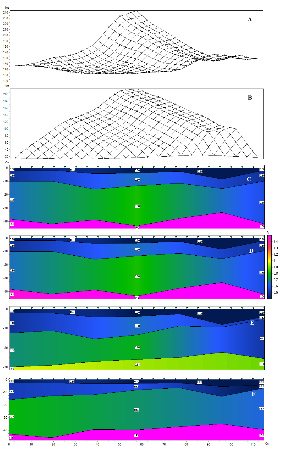
Рисунок 3 Пример инверсии синтетических данных отраженных и преломленных волн. A – расчетные годографы отраженных волн для модели C; B – расчетные годографы преломленных волн для модели C; C – оригинальная модель с отражающим основанием; D – результат совместной инверсии отраженных и преломленных волн; E - результат инверсии только преломленных волн; F - результат инверсии только отраженных волн.

   

Рисунок 2 демонстрирует результаты тестирования алгоритма для произвольной слоистой модели. Верхняя часть разреза представлена низкоскоростными осадочными образованиями, в основании лежат плотные скальные породы.

Система наблюдений состояла из 24 геофонов расположенных через 5 метров, с пунктом возбуждения на каждом.

Как видно из рисунка лучший результат получен при совместной инверсии данных отраженных и преломленных волн.

Тестирование производилось следующим образом:

На первом этапе инвертировались только времена первых вступлений для первого и второго типов модели. В качестве начального приближения использовалась горизонтально-слоистая среда с постоянным градиентом скоростей.

 На втором этапе скоростной разрез подбирался  по временам прихода отраженных волн для первого и второго типов модели. В качестве начального приближения использовалась горизонтально-слоистая среда с постоянным значением скорости.

На третьем  этапе проводилась совместная инверсия данных преломленных и отраженных волн. Как показал наш опыт, при работе с синтетическими данными, для достижения приемлемой невязки достаточно было трех-четырех итераций.

В заключение, полученные модели сравнивались с исходной.

Результаты тестирования для широкого класса моделей показали существенное улучшение точности определения параметров при совместной инверсии данных.

Также было проведено исследование влияния количества данных (рис.4) и шумовой составляющей (рис.5) на результат инверсии.

Рисунок 4  Пример инверсии синтетических данных отраженных и преломленных волн при полной и разреженных системах. A – 24 пункта возбуждения; B – 12 пунктов возбуждения; C – 6 пунктов возбуждения.

Анализ  результатов для систем наблюдений с различной плотностью пунктов возбуждения показал не слишком сильное снижение разрешающей способности.

Рисунок 5  Пример инверсии синтетических данных отраженных и преломленных волн при разном уровне шумовой составляющей.  A – оригинальная модель;. B – восстановленная, шум – 5 мсек; C - шум –10 мсек.  

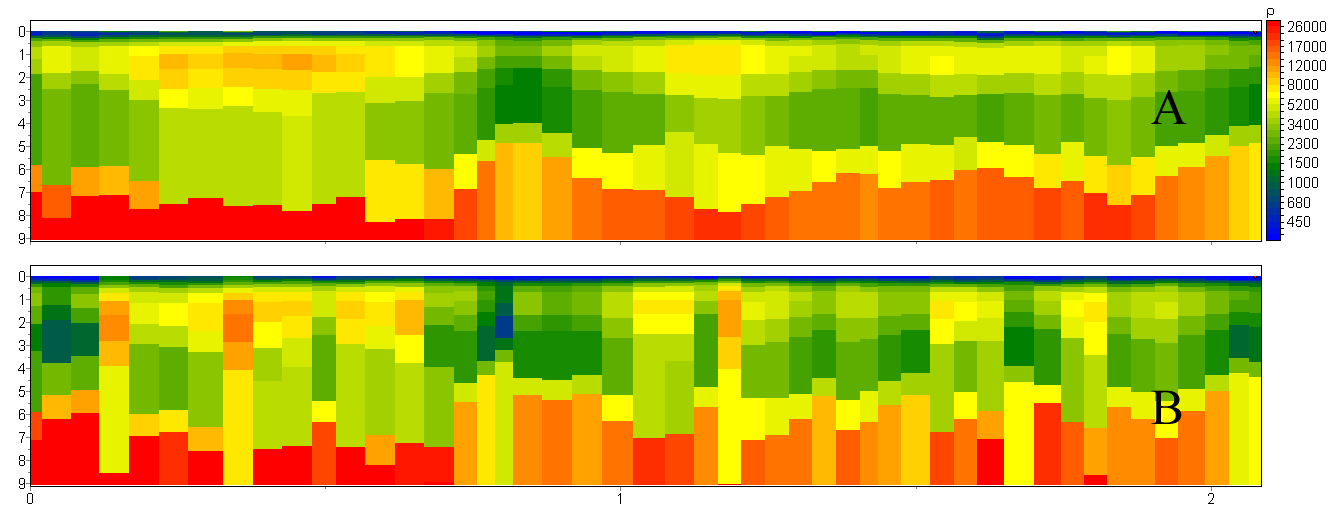
Алгоритм  совместной интерпретации  данных преломленных и отраженных волн реализован в программе ZondST2D  и в настоящее время проходит стадию тестирования на полевых материалах (рис.6).

Рисунок 6  Результат инверсии полевых данных (отражающая граница в основании разреза).  A – отраженные и преломленные;. B –только преломленные.

Для тестирования на полевых материалах использовалась система наблюдений с 48 геофонами через 2 метра и 9 пунктами возбуждения через 12 метров. Количество данных участвующих  в инверсии составляло: 362 - для рефрагированных,  160 - для отраженных волн. Конечная относительная невязка после инверсии  составила 5.2 процента.

 

Выводы

Предложенный в данной работе алгоритм может быть использован для обработки данных, как “большой”, так и  малоглубинной сейсморазведки. Совместная инверсия данных отраженных и преломленных волн существенно повышает качество результирующих скоростных разрезов.

Ссылки

1. Zhou B., Greenhalgh, S.A., Crosshole seismic inversion with normalized full-waveform amplitude data, Geophysics, 68, 2003.
2. J.W.D.Hobro, S.C.Singh,T.A.Minshull, Three-dimensional tomographic inversion of combined reflection and refraction seismic traveltime data. Geophysical Journal International, 152, 2003.
3. Moser T.J., Shortest path calculation of seismic rays, Geophysics, 56, 1991.
4. Constable S.,Parker R., Constable C. Occam's inversion: A practical algorithm for generating smooth models from electromagnetic sounding data, Geophysics 52, 1987.
   
   

Quality improvement of geoelectrical data interpretation

In recent years, the development of program-algorithmic base of electric exploration had an impact on the ways of field data interpretation. The software is responsible for the result. A formal approach to the data interpretation is a plus by many organizations, and departure from the standard of the count in every way possible suppressed. Such approach to interpretation is untenable because of some properties of inverse modeling. The visionless relevance of the interpreter to the algorithm output can lead to the inadequate results, which compromise geophysics in front of geologists. The inversion algorithm is like a “black box” – the quality of the results depends on the priori information.

Usually the interpretation begins with data analysis and primary data processing. Always there is a rule – “qualitative interpretation begins with the qualitative data”. It is impossible to overestimate the importance of qualitative analysis of observed data. Sometimes, even a small percentage of bad data can affect the resulting model. The dispersion of measurements is important for the data interpretation. Knowledge of dispersion estimator allows setting the correct weight of each measurement during inversion. It is useful to use iterative robust scheme for evaluation of data’s quality. These schemes should be applied in case of variation from the normal distribution of errors, spikes and etc. This algorithm applied to some sample data by different methods. For example, during interpretation of cross-borehole survey it is better to use robust scheme for the data in each of the source position separately.

Except industrial and instrumental method interferences is geological noise. It is known as P or C-effect. It appears when potential or current electrode falls on the local near-surface irregularity. The electric field strongly changes due to the irregularity. As a result, the sounding curve shifts without changing form (VES, MT). A lot of articles are dedicated to methods of controlling the geological noise. We propose the following algorithm to control the P-effect. It can be used during one-dimensional data interpretation.

Picture.1. Comparison of one-dimensional inversion results of electromagnetic sounding profile data according to the proposed (A) and standard (B) methods obtained with the use of ZondMT1D.

Parameter which modeling P-effect add to each curve during the two-dimensional interpretation of MTS data. Geological noise makes the strongest distortions in the data of cross-borehole tomography. During two- or three-dimensional inversion anomalous substance is formed in borehole environment. This substance is not associated with the real geological situation. Tramps, which are controlling by the borehole, separate the earth into loose area. In consequence, parameters are changed or the layers shift on different sides of the borehole. This complicates the geological interpretation of electrotomography results.

For solving this problem is proposed method, which allows to improve inversion results. The algorithm is to use a non-standard smoothing operator. The operator is constructed in such way that to produce through average of non-contiguous cells with borehole.

Picture.2. Comparison of inversion results of electromagnetic sounding synthetic data for model (A) according to the proposed (B) and standard (C) methods obtained with the use of ZondCHT.

During two-dimensional interpretation we should use the special algorithms, if the geoelectrical earth is complex. The complex earth is the earth, where angels of thin layers change or there are several structural levels within the one model. The standard inversion of this model is very rough and the result is not real. We developed the algorithm, which set up any averaging direction of smoothing operator for the different parts of model.

The next important way of quality improvement is adding the log data. The log data can be used in a qualitative or quantitative form. Resistivity log data allows locking or setting intervals range of changing in resistivity for cells along the borehole. Because of that the inversion results improved.

Picture.3. Comparison of inversion results of synthetic RMT data for model (A) with (B) and without (C) log data obtained with the use of ZondMT2D.

Undoubtedly, the best way of interpretation is the integration of geophysical methods. The some geophysical method is the most suitable for some modeling. To get all geological information, we should evaluate results jointly, because of possibility of each method to detect the different geological object. The quantitative integration method is based on special algorithm of focus inversion. The focus inversion is the modification of Occam, which allows to get sectionally-smooth parameterization. For an example, the cover thickness of rock foundation is known according the seismotomography. During electrotomography inversion the focus filter is used. This filter based on this boundary information.

Sometimes, model obtained by smooth inversion, we need to transform to structured geoelectrical model. This model consists of small amounts of objects. In order to do this we use polygonal interpretation. This is the more geological approach of data interpretation.

Picture.4. An example of structured geoelectrical model obtained with the use of ZondRes2dp.

In addition, there are algorithms of sequential interpretation of electrical and electromagnetic data. Result’s quality improvement depends on different sensitivity of electrical and electromagnetic methods to the parameters of geoelectrical models. Equivalent solution reduced due to the sequential interpretation.

There are many methods of data interpretation. This work is devoted to the methods, which are used more frequently during interpretation.

ProfileR_ZondRes2D

Resistivity imaging (ERT) with ZondRes2D